MS Excel- Data Validation

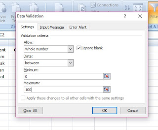
Data Validation: Data validation let the user to enter restricted data only,so it helps to avoid mistakes.For example: For a student, marks should be between 0 and 100. To put this restriction, select all the cells and click on 'Data validation' in 'Data tab' as shown in fig below:

 

Now select the data type under 'Allow' like in our case, we are selecting 'whole number'. Under 'Data', select the condition which we want to impose on the data, as  'between' is selected to restrict the values from 0 to 100 as shown in fig below:

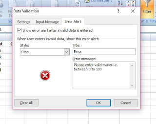
Now click on 'Error Alert' tab  and type the title under 'Title' and message under 'Error message' which we want to display, if user enter different data other than restricted.

Group and Ungroup: This option helps us to easily view and hide data in rows and columns. To do this select the rows and click on 'Group' option in 'Data' tab as shown in fig below:

After clicking the 'Group' option, data will be grouped as shown below and you can easily hide it .

Clicking on 'Ungroup' in 'Data' tab to simply undo the grouping.

Moreover it gets very easy with groups to perform specific functions on data belonging to common category.To understand this , consider an example, if we want to calculate average of students based on gender then

• select the number of rows
• click on 'subtotal' option in 'data' tab

• Set 'At each change' to 'Gender'
• Set 'Use function' to 'Average'
• Set 'Add subtotal to' to 'Total'
  
• Click on 'OK' button

It will give us average of 'Total' based on gender and total average too.

To learn about VLOOKUP function in MS Excel click here